Comparative Analysis of Colorization Techniques for Grayscale Images
In this project, we conducted a comparative analysis of colorization techniques for grayscale images, exploring methods such as Deep Learning, Support Vector Regression, and Probability-Based Methods.
Project Description
Four different methods for image colorization, namely support vector machines (SVM), Parzen windows (PWM), transfer learning, and conditional generative adversarial networks (cGAN) were implemented. The effectiveness of these methods was evaluated based on their ability to produce accurate and realistic colorized images, as well as their performance on various metrics such as mean absolute error (MAE), root mean square error (RMSE), peak signal-to-noise ratio (PSNR), and structural similarity index (SSIM).
Methods
The methods that we propose to use for the automatic image colorization are itemized below:
- Deep Learning
- Support Vector Regression
- Convolutional Neural Network
- Conditional Generative Adversarial Network
Dataset Information
Our dataset consists of 7,129 images depicting various scenes such as streets, buildings, mountains, glaciers, and trees. The dataset includes both color and grayscale versions of these images, facilitating direct comparisons across different methods.
Most images in the dataset have dimensions of 150 × 150 pixels, although some are smaller. We divided the dataset randomly, with 80% of the images designated as training data and the remaining 20% as testing data.
To ensure unbiased evaluation, the same distribution of training and testing images is maintained across all three methods. However, for SVR and PWM, only a subset of images is utilized for training due to scalability issues with larger training sets.
LAB Conversion
Accurately measuring color similarity and associating saturated colors with corresponding grayscale levels are crucial in image colorization.
In the classic RGB color space, every pixel is represented by three color values: Red, Green, and Blue. Hence, in an 8-bit image, each channel denoted (R, G, B) ranges from 0 to 255. Grayscale images, on the other hand, have only the intensity value for each pixel, resulting in a monochromatic image representation without any color information.
LAB 3D-space
By utilizing LAB color space, it has the ability to separate the luminance or lightness component (L channel) from the color components (a and b channels). The L channel solely represents the grayscale axis, capturing only the intensity or brightness information of the image from 0 to 100. On the other hand, the a and b channels encode the orthogonal color axes, representing the green-red and blue-yellow color information from -128 to 128, respectively.
Comparison & Validation Methods
Quantitative metrics such as MAE, RMSE, SSIM, and PSNR can assess structural differences by converting images to the YCbCr color space and using the Luma channel as the input. We will also employ cross-validation techniques, such as k-fold validation, which can help ensure unbiased performance assessment by training and testing the models on different subsets of the dataset.
Support Vector Regression
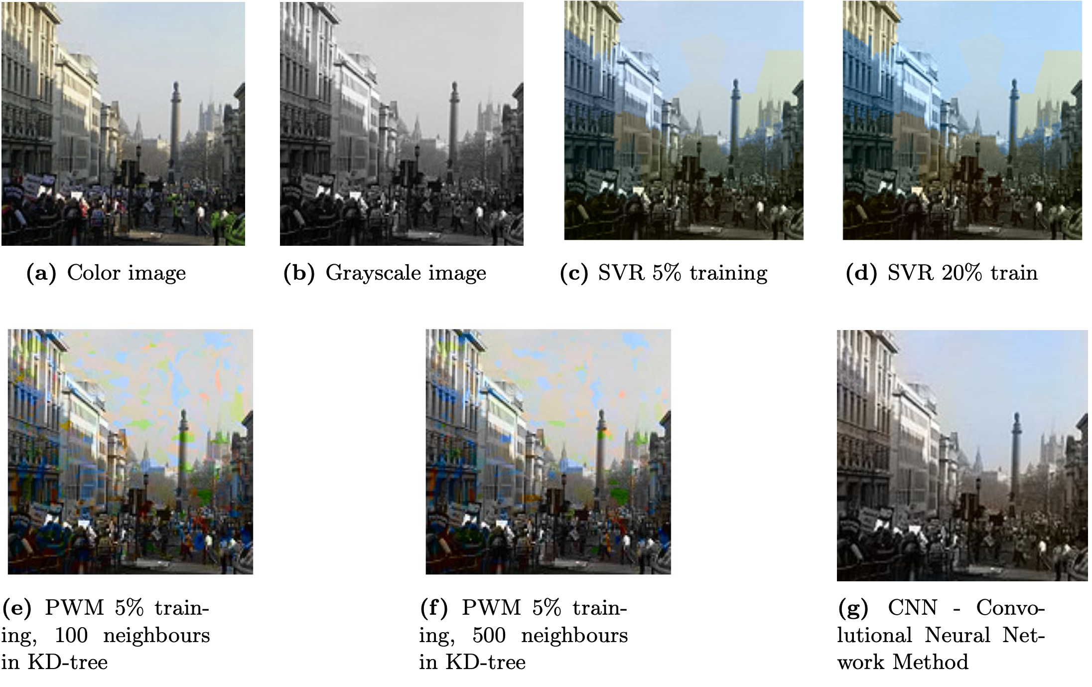
The Support Vector Regression (SVR) method utilizes a subset of the 80% training data due to SVR's poor scalability with the number of samples. Different percentages of training images (5%, 10%, and 20%) are employed to compare the method's quality for varying numbers of training images. During training, each colored image undergoes smoothing with a 3×3 Gaussian kernel (σ = 1), followed by segmentation using the SLIC superpixel algorithm to group similar grayscale brightness segments. After segmentation, the images are converted to LAB color space, and the scales of the a and b channels are adjusted to range between -1 and 1. A 2D Fourier transformation is applied to the L channel around the center of each segment, generating arrays for each segment along with the average a and b for every training image.
SVR model is trained using the sklearn.svm.SVR module, where the average a and b of each segment of each image are fitted against the array containing 2DFFT for each segment. The trained model is then used to predict the a and b channels of each segment in the test images. Attempts to implement Markov Random Field to smooth across adjacent segments were made but did not improve the results' quality and were consequently excluded from the process.
Parzen Window Methods & Spatial Coherence
In the exploration of Parzen Window Methods (PWM) for image colorization, the approach departs from traditional regression techniques to accommodate the natural multi-modality inherent in color selection. Drawing inspiration from existing literature, Parzen Window estimators are employed to learn local color predictors and variations directly from the training data, enabling the modeling of spatial coherency. This probabilistic, non-parametric method offers scalability and draws parallels with machine learning paradigms. The PWM framework integrates preprocessing steps involving the extraction of robust pixel features using the Scale-Invariant Feature Transform (SIFT) algorithm. Additionally, Principal Component Analysis (PCA) is applied to condense feature information, albeit with sub-optimal performance due to the algorithm's design and inherent information loss. Local descriptors, including pixel intensity and supplementary features, are computed for each grayscale pixel, facilitating the establishment of conditional probabilities between descriptors and colors in the LAB color space.
In contrast to conventional methods, spatial coherence in colorization is not determined by classic priors like edge or corner detection. Instead, the Parzen Window framework is leveraged to calculate the expected color variation for each pixel based on the gradient norms of the a and b channels. This approach ensures that color selection accounts for local and global influences, paving the way for the integration of Graph-cut algorithms. By combining color probability estimations and variations across neighborhoods, Graph-cut algorithms optimize image colorization by minimizing an objective function that balances local and global correctness. The optimization problem considers factors such as color probability reliability and estimated color variation at neighboring pixels, controlled by hyperparameters like ρ. This approach offers an alternative to diffusion methods and random walk techniques, providing comprehensive solutions for image colorization tasks.
Convolutional Neural Network
The Convolutional Neural Network (CNN) approach to grayscale image colorization employs transfer learning with the VGG16 model, a prominent deep learning architecture in computer vision tasks. CNNs, comprising convolutional layers, activation functions like ReLU, pooling layers, and fully-connected layers, excel in tasks such as image classification and object detection. Leveraging transfer learning, the pre-trained VGG16 model's feature extraction capabilities are utilized to enhance colorization performance significantly. By extracting features from grayscale images and retaining convolutional and pooling layers while discarding the fully-connected layers, the model can effectively detect essential patterns and color-related information. This transfer learning strategy enables the generation of high-quality colorized images with less reliance on extensive training data, thereby overcoming the limitations of isolated learning paradigms.
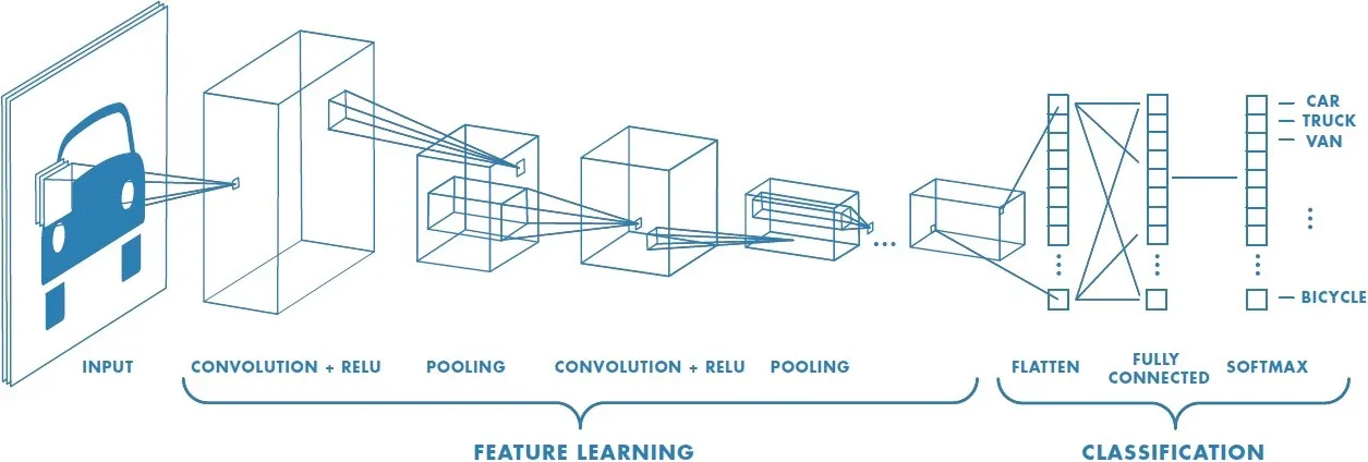
Convolutional Neural Network Architecture
During the training process, the model undergoes supervised learning with a dataset comprising grayscale images and corresponding colorized pairs. Data augmentation techniques, such as Keras' ImageDataGenerator, are employed to enhance the model's generalization capabilities. The grayscale input images are transformed into the LAB color space, with the L channel serving as input and the a and b channels as target color components. The model is trained using the Adam optimizer with the mean squared error (MSE) loss function, ensuring the minimization of differences between predicted and ground truth color components. The utilization of K-Fold Cross-Validation helps evaluate the model's performance across different subsets of the dataset, while early stopping mechanisms prevent overfitting. Despite achieving notable results, considerations for premature convergence suggest exploring more complex model architectures and augmenting the training dataset to capture a broader range of colorization patterns and scenarios effectively.
General Adversarial Network
The conditional general adversarial network (cGAN) represents a sophisticated approach to grayscale image colorization, offering greater control over the output compared to traditional GANs. Comprising a generator and discriminator, the cGAN operates by generating potential color images based on grayscale inputs and discerning their authenticity. The generator, functioning as a convolutional encoder decoder (CAE), employs multiple Conv2D layers to process the input grayscale images and output corresponding colored images. Meanwhile, the discriminator, a convolutional neural network (CNN), distinguishes between real and generated images, facilitating adversarial training between the two modules. The sequential training process involves initially generating fake images, which are subsequently evaluated by the discriminator alongside a batch of real images. The generator is then trained based on the feedback from the cGAN, while the discriminator remains unchanged during this phase, ensuring a dynamic training process that iteratively refines the colorization model.
The effectiveness of cGANs in grayscale image colorization is underscored by their capacity to incorporate additional information and fine-tune the output based on specified criteria. Notably, the development of advanced frameworks like pix2pix, trained on extensive datasets such as ImageNet, highlights the potential of deep learning networks in this domain. The utilization of large-scale datasets containing millions of images underscores the significance of data volume in optimizing the performance of algorithms like cGANs. This underscores the importance of dataset size and diversity in training robust and effective colorization models, hinting at the considerable computational resources and data infrastructure required for implementing advanced algorithms in grayscale image colorization tasks.
Key differences
One of the key differences noted in this paper was the different requirements for training volume between the deep learning methods and the non-deep learning methods. The SVM, for instance, needed to be trained at a reduced value of already limited pictures, whereas the limited available images in the dataset actually reduced the effectiveness of the transfer learning network, potentially contributing towards its premature convergence.
Results
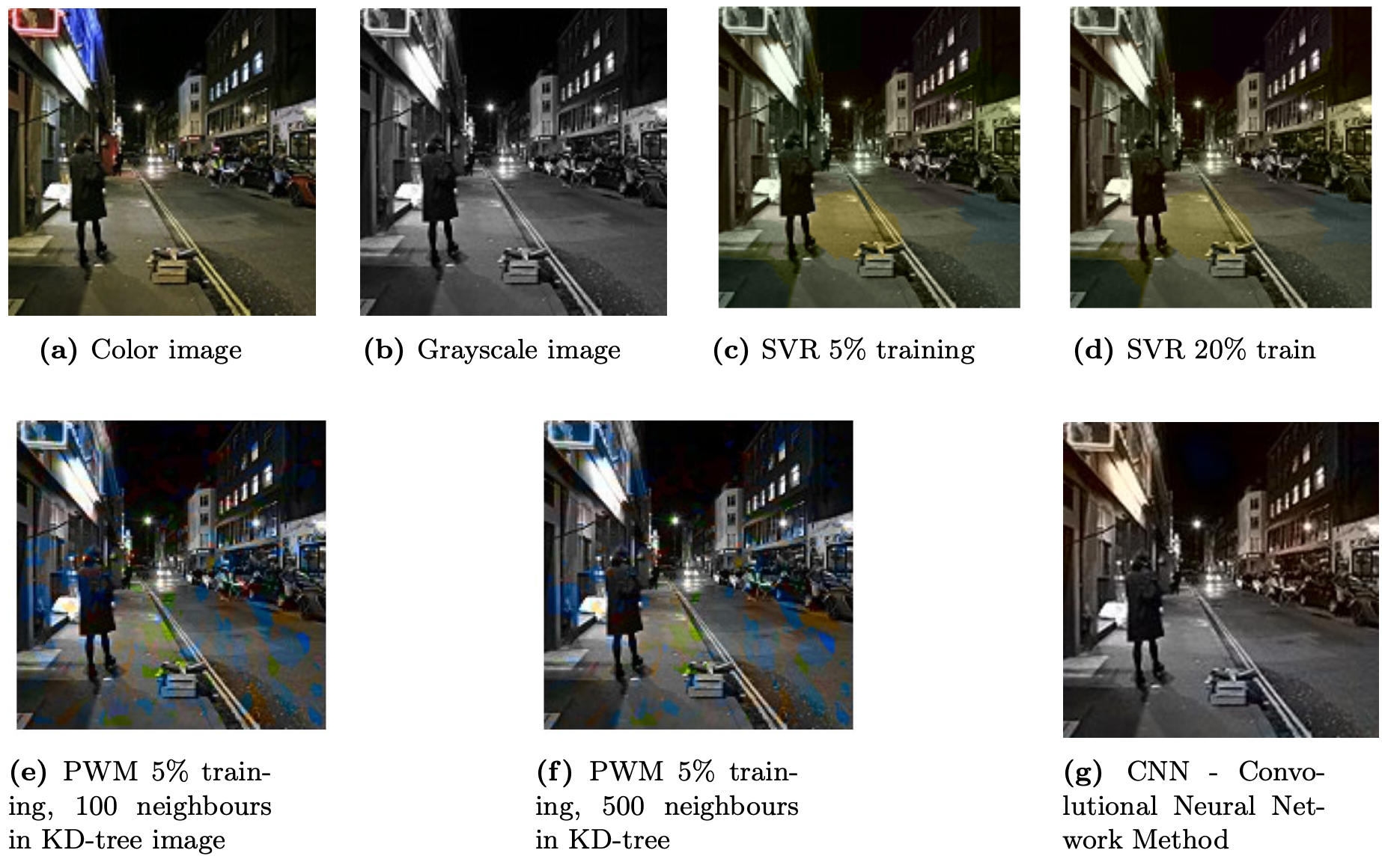
Test Image No. 16
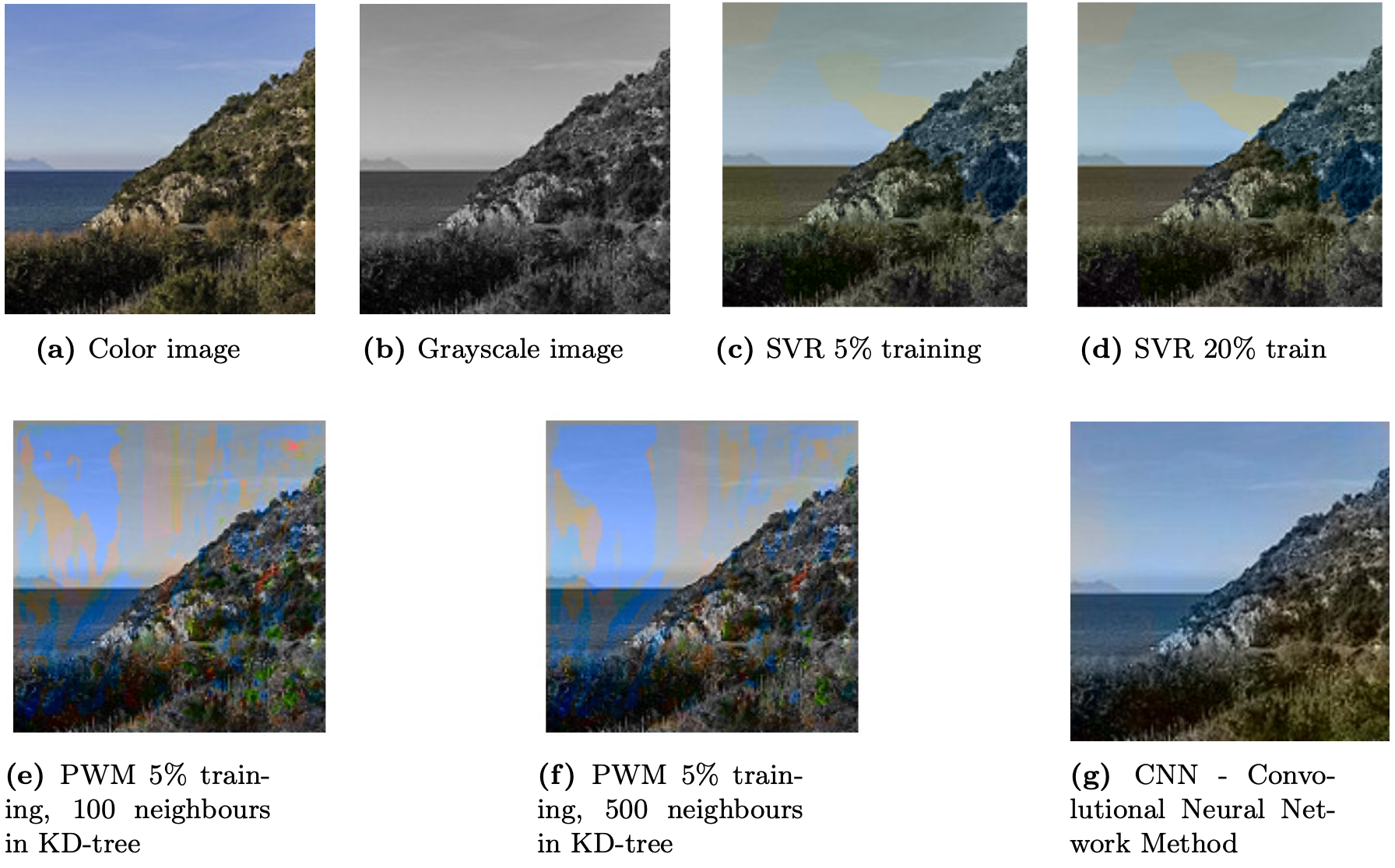
Test Image No. 17
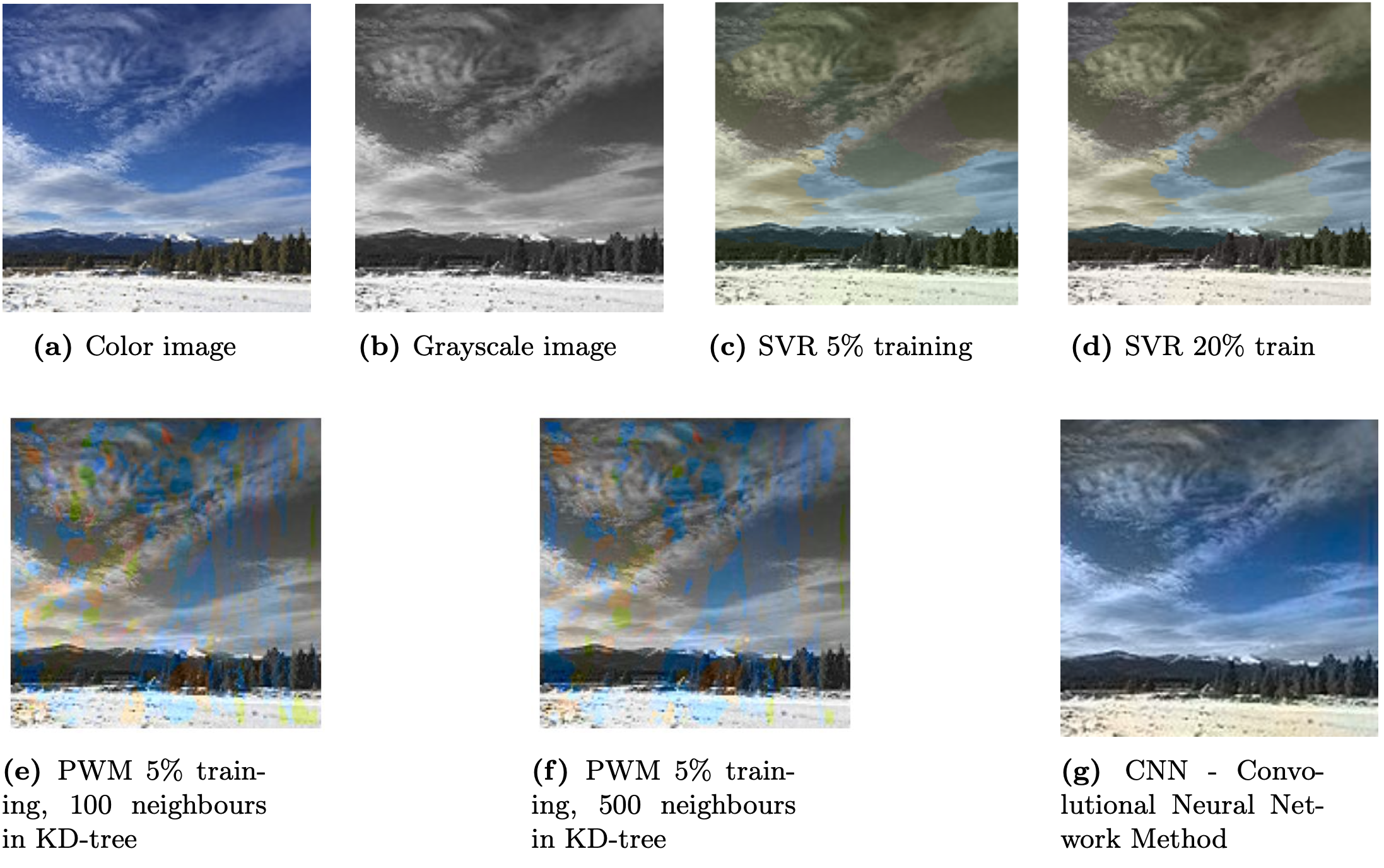
Test Image No. 18
Test Image No. 19
The evaluation of colorization methods highlights distinct performance characteristics across different models. SVR demonstrates suitability for smaller datasets due to its poor scalability with increasing data size, yielding blocky color outputs. However, the method struggles with nuanced color transitions and texture bleeding, particularly evident in cloudy sky scenarios. In contrast, the Bayesian Parzen Window method exhibits patchiness and inconsistent coloration due to the absence of smoothing algorithms, emphasizing the need for refinement in handling color coherence. Adjusting hyperparameters like K for KD-tree structures shows limited impact on output quality, suggesting optimization opportunities in pixel selection strategies.
CNN deep learning neural network's performance varies notably across nature and cityscape images, reflecting the diverse complexities inherent in each scene type. While nature images offer clearer features and color variations, cityscapes pose challenges with intricate details and uniform textures. Strategies such as data augmentation, domain-specific architectural adjustments, and user feedback hold promise for enhancing cityscape image colorization accuracy. Overall, the comparative analysis underscores the importance of tailored approaches to address the unique challenges posed by different image contexts and the potential for further refinement in colorization methodologies.
Comparison in Metrics Between Methods
| SVR | SVR-STD | PWM | PWM-STD | CNN | CNN-STD | |
|---|---|---|---|---|---|---|
| Mean Absolute Error A | 7.23 | 4.42 | 6.64 | 2.58 | 5.75 | 4.49 |
| Mean Absolute Error B | 15.6 | 7.02 | 16.6 | 8.40 | 13.1 | 6.61 |
| Root Mean Square Error A | 8.61 | 4.97 | 9.37 | 3.26 | 7.35 | 5.14 |
| Root Mean Square Error B | 18.6 | 7.92 | 21.6 | 8.83 | 16.1 | 7.25 |
| SSIM | 0.91 | 0.06 | 0.74 | 0.10 | 0.94 | 0.05 |
| PSNR | 29.9 | 0.81 | 19.1 | 3.26 | 23.0 | 3.83 |
Conclusion
Broadly, two different techniques were applied: deep learning and non-deep learning methods. The SVR required reduced training volume compared to other methods, but the limited available images reduced the effectiveness of the transfer learning network.
Images colorized by the Probabilistic-diffusion and SVR methods exhibited color issues upon generation. Larger training datasets did not always correlate with better results, raising questions about method appropriateness for large datasets.
The CNN deep learning model outperformed others on most metrics, indicating the need for further research. However, other techniques may be more beneficial with limited data. The cGAN, though not fully implemented, warrants further exploration.
Next Steps
For SVR, improving scalability and quality through sklearn.svm.LinearSVR and Markov Random Fields implementation is suggested. PWM could benefit from pixel-to-section level approaches and coherence optimization. CNN requires fine-tuning, hyperparameter tuning, data augmentation, and diverse dataset incorporation to enhance colorization. cGAN evaluation against other methods and consideration of training data quantity are essential for further development.
Group
- Gummesen, Thomas Skøtt
- Lam, Hui Yin (Henry)
- Pepping, Bartholomeus Diederik Rasmussen
- Magne Egede
You can read our written report here.
Code on GitHub: https://github.com/HenryLamBlog/Colorization